McCall Search Model

David Evans

2026-04-20

Model Setup

The Environment

The McCall Search Model

• Worker lives for \(T\) (possibly infinite) periods
• Can be either unemployed or employed
• Discounts the future at rate \(\beta\)

• If unemployed: receives a wage offer \(\bar w_j\) with probability \(p_j\)

• Two choices each period:
  • Accept: receive wage \(\bar w_j\) and become employed
  • Reject: receive unemployment benefits \(c\) and remain unemployed

Objective

• Worker maximizes expected discounted lifetime income:

\[ \mathbb{E} \sum_{t=0}^T \beta^t y_t \]

where \(y_t = c\) if unemployed and \(y_t = w_t\) if employed

• Can be fired with probability \(\alpha\) at the end of each period (begin by assuming \(\alpha = 0\))

The Decision Tree

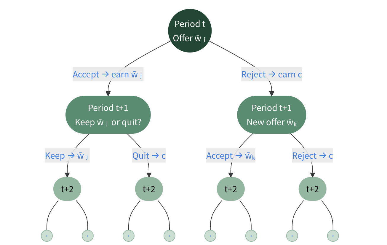
• \(2^n\) possible paths after \(n\) periods — how to solve this efficiently?

Employed vs. Unemployed

• An unemployed worker with wage offer \(\bar w_j\) can reject the offer, receive \(c\), and draw a new offer next period

• Or accept the offer, receive \(\bar w_j\), and be employed next period at wage \(\bar w_j\)

• An employed worker with wage \(\bar w_j\) can quit, receive \(c\), and draw a new offer next period

• Or continue to work, receive \(\bar w_j\), and be employed next period at wage \(\bar w_j\)

Insight

An employed worker deciding whether to keep wage \(\bar w_j\) faces the same problem as an unemployed worker who just received offer \(\bar w_j\).

Setup Parameters

using Plots
using LinearAlgebra

β = 0.95       # discount factor
S = 50         # number of possible wage offers
w̄ = LinRange(1., 10., S)   # wage offers
p = ones(S)/S  # equal probability of each wage
c = 3.         # unemployment benefit

3.0

Roadmap

What We’ll Cover

1. Finite Horizon — solve the model by backward induction
2. Solving with Functions — package code into reusable functions
3. Infinite Horizon — take \(T \to \infty\) with value function iteration
4. Organizing with Structs — group parameters using Julia structs
5. Firing Risk — extend the model with job separation
6. Comparative Statics — how do policy changes affect outcomes?

Finite Horizon

One Period Problem

Value with One Period Left

• What is the value of an unemployed worker who receives offer \(\bar w_j\) in the last period?

\[ V_{1,j} = \max\left\{ \bar w_j,\; c \right\} \]

• \(V_{1,j}\) = value with one period left and wage offer \(\bar w_j\)

Computing the One-Period Value

V1 = max.(w̄, c)   # V1[j] = max(w̄[j], c) for each j

50-element Vector{Float64}:
  3.0
  3.0
  3.0
  3.0
  3.0
  3.0
  3.0
  3.0
  3.0
  3.0
  ⋮
  8.53061224489796
  8.714285714285714
  8.89795918367347
  9.081632653061224
  9.26530612244898
  9.448979591836736
  9.63265306122449
  9.816326530612246
 10.0

Plotting the One-Period Value

scatter(w̄, V1, label="V₁", legend=:topleft)
xlabel!("Wage")
ylabel!("Value (1 period left)")

Expected Value of a Random Offer

• Define \(Q_1\) as the expected value of a random wage offer with 1 period left:

\[ Q_1 = \sum_s p_s V_{1,s} = p \cdot V_1 \]

Q1 = dot(p, V1)

5.737959183673469

Two Period Problem

Value with Two Periods Left

• Value of accepting offer \(\bar w_s\):

\[ \bar w_s + \beta V_{1,s} \]

• Value of rejecting the offer:

\[ c + \beta Q_1 \]

• The worker chooses the best option:

\[ V_{2,s} = \max\left\{ \bar w_s + \beta V_{1,s},\; c + \beta Q_1 \right\} \]

Computing Two-Period Values

V2accept = w̄ + β*V1       # value of accepting for each wage
V2reject = c + β*Q1        # value of rejecting (a scalar)
V2 = max.(V2accept, V2reject)

50-element Vector{Float64}:
  8.451061224489795
  8.451061224489795
  8.451061224489795
  8.451061224489795
  8.451061224489795
  8.451061224489795
  8.451061224489795
  8.451061224489795
  8.451061224489795
  8.451061224489795
  ⋮
 16.634693877551022
 16.99285714285714
 17.351020408163265
 17.709183673469386
 18.067346938775508
 18.425510204081633
 18.783673469387757
 19.14183673469388
 19.5

Plotting the Two-Period Value

scatter(w̄, V2, label="V₂", legend=:topleft)
scatter!(w̄, V1, label="V₁")
xlabel!("Wage")
ylabel!("Value")

Expected Value with Two Periods

Q2 = dot(p, V2)

11.970484897959183

• This can be used in the 3 period problem

• And then the 4-period problem

• And then the 5 period problem

General \(t\)-Period Problem

The Bellman Equation

• For a worker with \(t\) periods left and wage offer \(\bar w_s\):

• Value of accepting: \(\bar w_s + \beta V_{t-1,s}\)

• Value of rejecting: \(c + \beta Q_{t-1}\)

\[ \boxed{V_{t,s} = \max\left\{ \bar w_s + \beta V_{t-1,s},\; c + \beta Q_{t-1} \right\}} \]

Backward Induction

Solution Strategy

We solve backwards from the last period: compute \(V_1\), then \(V_2\), then \(V_3\), and so on.

Solving with a For Loop

T = 50                                # number of periods the worker lives
S = length(w̄)                        # number of possible wages
V = zeros(T, S)                       # V[t,s] = value with t periods left, offer s
Q = zeros(T)                          # Q[t] = expected value of random offer

V[1, :] = max.(c, w̄)                 # base case: last period, just pick max
Q[1] = dot(p, V[1, :])               # expected value in last period

for t in 2:T                          # build up from t=2 to t=T
    Vaccept = w̄ + β*V[t-1, :]        # wage today + discounted continuation
    Vreject = c + β*Q[t-1]            # benefits today + discounted random offer
    V[t, :] = max.(Vaccept, Vreject)  # optimal choice for each wage
    Q[t] = dot(p, V[t, :])           # update expected value
end

Plotting Value Functions

plot()
for t in [1, 10, 20, 30, 50]
    scatter!(w̄, V[t, :], label="t = $t")
end
xlabel!("Wage")
ylabel!("Value")

• More periods left \(\rightarrow\) higher value (more opportunities to find a good wage)

Solving with Functions

The Bellman Iteration Function

iterateBellman: Pseudocode

• Wrap the single-step Bellman update in a reusable function

function iterateBellman(V, Q, β, p, w̄, c)     # V, Q from next period
    # Compute value of accepting each wage offer
    # Compute value of rejecting (same for all wages)
    # Pick the better option for each wage
    # Compute expected value of a random offer
    # Return updated V, Q, and acceptance decision C
end

iterateBellman: Accept vs. Reject

• First, compute the value of each option:

function iterateBellman(V, Q, β, p, w̄, c)
    V_accept = w̄ .+ β .* V                       # w̄[s] + β*V[s] for each wage s
    V_reject = c  + β  * Q                        # c + β*Q (same for all wages)
    # ...
end

• V_accept is a vector — one value for each wage offer
• V_reject is a scalar — same for all wages (the outside option)
• The dot in w̄ + β * V broadcasts element-wise: each wage \(\bar{w}_s\) plus the discounted continuation \(\beta V_s\)

iterateBellman: Full Function

function iterateBellman(V, Q, β, p, w̄, c)     # V, Q from next period
    V_accept = w̄ .+ β .* V                       # w̄[s] + β*V[s] for each wage s
    V_reject = c  + β  * Q                        # c + β*Q (same for all wages)
    V_new = max.(V_accept, V_reject)            # pick the better option
    Q_new = dot(p, V_new)                       # expected value of random offer
    C = V_accept .>= V_reject                   # 1 = accept, 0 = reject
    return (V=V_new, Q=Q_new, C=C)               # named tuple of results
end

iterateBellman (generic function with 1 method)

Named Tuple Returns

• Our functions return named tuples instead of plain tuples:

return (V=V_new, Q=Q_new, C=C)

• Two ways to access the results:

ret = iterateBellman(V, Q, β, p, w̄, c)
ret.V                      # access by name — self-documenting
ret.C                      # no need to remember the order

V, Q, C = iterateBellman(V, Q, β, p, w̄, c) # destructuring still works!

Why Named Tuples?

With 3–4 return values, it’s easy to forget the order. Named tuples let you access results by name — no more guessing which output is which.

solveMcCall: Pseudocode

function solveMcCall(β, p, w̄, c, T)           # T = number of periods
    # Allocate storage for V, Q, and C
    # Set base case: V with 1 period left
    # Loop from t=2 to T, calling iterateBellman each step
    # Return named tuple with V, Q, C
end

solveMcCall: Base Case

• Start from the last period (\(t = 1\)):

function solveMcCall(β, p, w̄, c, T)
    S = length(w̄)
    V = zeros(T, S);  Q = zeros(T);  C = zeros(Int, T, S)

    V[1, :] = max.(w̄, c)                      # just pick the higher payoff
    Q[1] = dot(p, V[1, :])                     # expected value of random offer
    C[1, :] = w̄ .>= c                         # accept if wage ≥ benefits
    # ...
end

• V[1, :] stores the value function with 1 period left — simply \(\max(\bar{w}_s, c)\)
• Q[1] is the expected value of a random offer: \(Q_1 = p \cdot V_1\)

solveMcCall: Full Function

function solveMcCall(β, p, w̄, c, T)           # T = number of periods
    S = length(w̄)                              # number of wage offers
    V = zeros(T, S);  Q = zeros(T);  C = zeros(Int, T, S)  # allocate storage

    V[1, :] = max.(w̄, c)                      # base case: V with 1 period left
    Q[1] = dot(p, V[1, :])                     # expected value with 1 period left
    C[1, :] = w̄ .>= c                         # accept if wage ≥ benefits

    for t in 2:T                                # iterate from 2 to T periods
        V[t, :], Q[t], C[t, :] = iterateBellman(V[t-1, :], Q[t-1], β, p, w̄, c)
    end                                         # uses previous period's solution
    return (V=V, Q=Q, C=C)                       # return as named tuple
end

solveMcCall (generic function with 1 method)

Value Functions for 100 Periods

V, Q, C = solveMcCall(β, p, w̄, c, 100)       # solve for T = 100 periods
plot()                                          # initialize empty plot
for t in [1, 2, 3, 10, 20, 50, 100]            # plot selected periods
    scatter!(w̄, V[t, :], label="t = $t")       # add value function for period t
end
xlabel!("Wage")                                 # label axes
ylabel!("Value of Offer")

• Note: little difference between \(V_{50}\) and \(V_{100}\) — the value function is converging

Infinite Horizon

From Finite to Infinite

Taking the Limit

• As \(t \to \infty\), the value function converges: \(V_{t,s} \approx V_{t+1,s}\)
• The problem faced today is the same as the problem faced tomorrow

• Taking the limit of the Bellman equation:

\[ V_s = \max\left\{ \bar w_s + \beta V_s,\; c + \beta Q \right\} \]

where \(Q = p \cdot V\)

The Fixed Point Problem

Fixed Point

The infinite horizon value function satisfies a fixed point equation: \(V\) appears on both sides.

• We solve by iterating: guess \(V\), apply the Bellman equation, repeat until \(V\) stops changing

Value Function Iteration

V = max.(w̄, c)                                    # initial guess for V
C = w̄ .>= c                                      # initial guess for policy
Q = dot(p, V)                                      # initial guess for Q

dist = 1.0                                         # initialize distance
while dist > 1e-10                                 # loop until convergence
    V_new, Q_new, C = iterateBellman(V, Q, β, p, w̄, c)  # one Bellman step
    dist = norm(V - V_new, Inf)                     # max |V_new - V| across wages
    V = V_new                                       # replace old V with new
    Q = Q_new                                       # replace old Q with new
end

Convergence Speed

Why Does VFI Converge?

The Bellman operator is a contraction mapping with modulus \(\beta\).

• After \(n\) iterations, the error is at most \(\beta^n \|V_0 - V^*\|\)
• With \(\beta = 0.95\), each iteration shrinks the error by 5%
• Convergence is geometric — fast enough for most applications

The Infinite Horizon Solution

scatter(w̄, V, label="Value", legend=:topleft)
xlabel!("Wage")
ylabel!("Value")

The Optimal Policy

scatter(w̄, C, label="Accept (1) / Reject (0)", legend=:topleft)
xlabel!("Wage")
ylabel!("Choice")

The Reservation Wage

Reservation Wage

The optimal policy is a threshold rule: accept any wage above a cutoff (the reservation wage) and reject wages below it.

Computing the Reservation Wage

w_res = w̄[findfirst(C .== 1)]    # first wage where worker accepts
println("Reservation wage: ", round(w_res, digits=2))

Reservation wage: 7.98

• The worker rejects any offer below this threshold and waits for a better one

solveMcCall (Infinite Horizon): Pseudocode

function solveMcCall(β, p, w̄, c)               # no T argument → infinite horizon
    # Initialize V, Q, C with simple guesses
    # Loop: apply iterateBellman until V stops changing
    # Return named tuple with V, Q, C
end

solveMcCall (Infinite Horizon): The Convergence Loop

• The key difference from the finite-horizon solver: we iterate until convergence instead of a fixed number of steps

    dist = 1.0                                  # initialize distance
    while dist > 1e-10                          # loop until convergence
        V_new, Q_new, C = iterateBellman(...)   # one Bellman step
        dist = norm(V - V_new, Inf)             # max |V_new - V| across wages
        V = V_new;  Q = Q_new                   # replace old with new
    end

• norm(V - V_new, Inf) computes the sup-norm: the largest absolute change across all wages
• When this is smaller than \(10^{-10}\), the value function has converged

solveMcCall (Infinite Horizon): Full Function

function solveMcCall(β, p, w̄, c)               # no T argument → infinite horizon
    V = max.(w̄, c);  C = w̄ .>= c;  Q = dot(p, V)  # initial guesses

    dist = 1.0                                  # initialize distance
    while dist > 1e-10                          # iterate until convergence
        V_new, Q_new, C = iterateBellman(V, Q, β, p, w̄, c)  # Bellman step
        dist = norm(V - V_new, Inf)             # check max absolute difference
        V = V_new;  Q = Q_new                   # update V and Q
    end
    return (V=V, Q=Q, C=C)                      # return as named tuple
end

solveMcCall (generic function with 2 methods)

Organizing with Structs

Why Structs?

The Problem with Many Arguments

• Our solver: solveMcCall(β, p, w̄, c) — 4 separate arguments
• With firing: solveMcCallFiring(β, p, w̄, c, α) — 5 arguments
• As models grow, we pass more and more parameters to every function

• Easy to mix up argument order, hard to read, tedious to change

• Solution: bundle all model parameters into a single object

Structs as Blueprints

• A struct defines a new data type that groups related data together
• Think of it as a blueprint or template:
  • The struct defines what fields a model needs (β, w̄, p, c, …)
  • An instance fills in specific values for those fields

Analogy

McCallModel is like a blank form: “every McCall model needs a β, w̄, p, and c.” Creating an instance fills in the blanks with specific numbers.

Defining a Struct

The @kwdef Macro

• Julia’s built-in @kwdef macro provides two useful features:
  • Define structs with default values
  • Combined with destructuring (; ...), extract fields into local variables

Defining McCallModel

@kwdef struct McCallModel
    β::Float64 = 0.95                                   # discount factor
    S::Int = 50                                          # number of wage offers
    w̄::Vector{Float64} = collect(LinRange(1., 10., S))  # wage grid
    p::Vector{Float64} = ones(S)/S                       # probabilities
    c::Float64 = 3.0                                     # unemployment benefit
    α::Float64 = 0.0                                     # firing probability
end

McCallModel

• @kwdef lets every field have a default value

Creating Instances

• Use all defaults:

m = McCallModel()

McCallModel(0.95, 50, [1.0, 1.183673469387755, 1.3673469387755102, 1.5510204081632653, 1.7346938775510203, 1.9183673469387754, 2.1020408163265305, 2.2857142857142856, 2.4693877551020407, 2.6530612244897958  …  8.346938775510203, 8.53061224489796, 8.714285714285714, 8.89795918367347, 9.081632653061224, 9.26530612244898, 9.448979591836736, 9.63265306122449, 9.816326530612246, 10.0], [0.02, 0.02, 0.02, 0.02, 0.02, 0.02, 0.02, 0.02, 0.02, 0.02  …  0.02, 0.02, 0.02, 0.02, 0.02, 0.02, 0.02, 0.02, 0.02, 0.02], 3.0, 0.0)

• Change one parameter — only specify what’s different:

m_generous = McCallModel(c = 5.0)

McCallModel(0.95, 50, [1.0, 1.183673469387755, 1.3673469387755102, 1.5510204081632653, 1.7346938775510203, 1.9183673469387754, 2.1020408163265305, 2.2857142857142856, 2.4693877551020407, 2.6530612244897958  …  8.346938775510203, 8.53061224489796, 8.714285714285714, 8.89795918367347, 9.081632653061224, 9.26530612244898, 9.448979591836736, 9.63265306122449, 9.816326530612246, 10.0], [0.02, 0.02, 0.02, 0.02, 0.02, 0.02, 0.02, 0.02, 0.02, 0.02  …  0.02, 0.02, 0.02, 0.02, 0.02, 0.02, 0.02, 0.02, 0.02, 0.02], 5.0, 0.0)

Creating Instances

• Change multiple parameters:

m_patient = McCallModel(β = 0.99, c = 4.0)

McCallModel(0.99, 50, [1.0, 1.183673469387755, 1.3673469387755102, 1.5510204081632653, 1.7346938775510203, 1.9183673469387754, 2.1020408163265305, 2.2857142857142856, 2.4693877551020407, 2.6530612244897958  …  8.346938775510203, 8.53061224489796, 8.714285714285714, 8.89795918367347, 9.081632653061224, 9.26530612244898, 9.448979591836736, 9.63265306122449, 9.816326530612246, 10.0], [0.02, 0.02, 0.02, 0.02, 0.02, 0.02, 0.02, 0.02, 0.02, 0.02  …  0.02, 0.02, 0.02, 0.02, 0.02, 0.02, 0.02, 0.02, 0.02, 0.02], 4.0, 0.0)

Accessing Fields

• Use dot notation to access any field:

m.β

0.95

m.c

3.0

m.w̄[1:5]

5-element Vector{Float64}:
 1.0
 1.183673469387755
 1.3673469387755102
 1.5510204081632653
 1.7346938775510203

Destructuring Fields

• Inside a function, destructuring extracts fields into local variables:

(; β, p, w̄, c) = m
β

0.95

Why Destructuring?

Instead of writing m.β, m.p, m.w̄, m.c everywhere in our math, destructuring gives us clean local variable names — the code looks the same as before.

Rewriting with Structs

iterateBellman with a Struct

function iterateBellman(m::McCallModel, V, Q)   # V, Q from next period + model
    (; β, p, w̄, c) = m                     # extract parameters
    V_accept = w̄ + β * V                       # w̄[s] + β*V[s] for each wage s
    V_reject = c + β * Q                        # c + β*Q (same for all wages)
    V_new = max.(V_accept, V_reject)            # pick the better option
    Q_new = dot(p, V_new)                       # expected value of random offer
    C = V_accept .>= V_reject                   # 1 = accept, 0 = reject
    return (V=V_new, Q=Q_new, C=C)             # named tuple of results
end

iterateBellman (generic function with 2 methods)

• Now only 3 arguments instead of 6 — the model carries the rest

solveMcCall with a Struct

function solveMcCall(m::McCallModel)            # takes a single McCallModel
    (; β, p, w̄, c) = m                     # extract parameters
    V = max.(w̄, c);  C = w̄ .>= c;  Q = dot(p, V)

    dist = 1.0
    while dist > 1e-10
        V_new, Q_new, C = iterateBellman(m, V, Q)  # pass the model
        dist = norm(V - V_new, Inf)
        V = V_new;  Q = Q_new
    end
    return (V=V, Q=Q, C=C)                      # named tuple
end

solveMcCall (generic function with 3 methods)

Using the Struct Version

m = McCallModel()
sol = solveMcCall(m)       # returns a named tuple

(V = [158.24988988232073, 158.24988988232073, 158.24988988232073, 158.24988988232073, 158.24988988232073, 158.24988988232073, 158.24988988232073, 158.24988988232073, 158.24988988232073, 158.24988988232073  …  166.93877550863462, 170.61224489635495, 174.28571428407582, 177.9591836717961, 181.63265305951697, 185.3061224472373, 188.97959183495811, 192.65306122267842, 196.32653061039926, 199.9999999981196], Q = 163.42093671832137, C = Bool[0, 0, 0, 0, 0, 0, 0, 0, 0, 0  …  1, 1, 1, 1, 1, 1, 1, 1, 1, 1])

sol.V[1:5]                 # access value function by name

5-element Vector{Float64}:
 158.24988988232073
 158.24988988232073
 158.24988988232073
 158.24988988232073
 158.24988988232073

scatter(m.w̄, sol.V, label="Value", legend=:topleft)
xlabel!("Wage")
ylabel!("Value")

Using the Struct Version

Multiple Dispatch

Julia’s Multiple Dispatch

Julia picks which solveMcCall to call based on the argument type:

• solveMcCall(m) where m::McCallModel → struct version
• solveMcCall(β, p, w̄, c) → original version

Both work! Julia dispatches to the right method automatically.

Hazard Rates

What is the Hazard Rate?

• The hazard rate is the probability of leaving unemployment each period:

\[ h = p_1 C_1 + p_2 C_2 + \cdots + p_S C_S = p \cdot C \]

• \(C_s = 1\) if the worker accepts wage \(\bar w_s\), 0 otherwise

Computing the Hazard Rate

m = McCallModel()
sol = solveMcCall(m)
dot(m.p, sol.C)            # hazard rate using named tuple access

0.23999999999999996

Expected Unemployment Duration

• If the hazard rate is \(h\), the expected duration of unemployment is:

\[ \mathbb{E}[\text{duration}] = \frac{1}{h} \]

h = dot(m.p, sol.C)
println("Hazard rate: ", round(h, digits=3))
println("Expected duration: ", round(1/h, digits=1), " periods")

Hazard rate: 0.24
Expected duration: 4.2 periods

Hazard Rate and Unemployment Benefits

• How does the hazard rate change with \(c\)?

cvalues = LinRange(0, 5, 100)                       # grid of c values to try
hvalues = zeros(length(cvalues))                    # store hazard rate for each c
for i in 1:length(cvalues)                          # loop over each c
    sol = solveMcCall(McCallModel(c=cvalues[i]))    # create model, solve
    hvalues[i] = dot(p, sol.C)                      # compute hazard rate p⋅C
end
plot(cvalues, hvalues, linewidth=2, label="Hazard Rate", legend=:topright)
xlabel!("Unemployment Benefits (c)")                # label axes
ylabel!("Hazard Rate")

• Higher \(c\) \(\rightarrow\) worker is more selective \(\rightarrow\) lower hazard rate

Firing

Model with Firing

Adding Firing Risk

• Now suppose an employed worker gets fired with probability \(\alpha\) at end of period
• When fired, immediately draws a new wage offer

• Let \(U_t\) = value of being unemployed with \(t\) periods left:

\[ U_t = c + \beta Q_{t-1} \]

Value of Accepting with Firing Risk

• Value of accepting offer \(\bar w_s\):

\[ \bar w_s + \beta\left[(1-\alpha) V_{t-1,s} + \alpha U_{t-1}\right] \]

The Bellman Equation with Firing

\[ \boxed{V_{t,s} = \max\left\{ \bar w_s + \beta\left[(1-\alpha) V_{t-1,s} + \alpha U_{t-1}\right],\; U_t \right\}} \]

Effect of Firing

Firing risk reduces the value of accepting a job, since employment is no longer permanent.

Bellman Iteration with Firing

function iterateBellmanFiring(m::McCallModel, V, Q, U)  # model first
    (; β, p, w̄, c, α) = m                  # extract all parameters
    V_accept = w̄ + β * ((1-α)*V .+ α*U)        # keep job w.p. 1-α, fired w.p. α
    U_new = c + β * Q                            # unemployment: benefits + random offer
    V_new = max.(V_accept, U_new)                # pick the better option
    Q_new = dot(p, V_new)                        # expected value of random offer
    C = V_accept .>= U_new                       # 1 = accept, 0 = reject
    return (V=V_new, Q=Q_new, U=U_new, C=C)     # named tuple with U
end

iterateBellmanFiring (generic function with 1 method)

• 4 arguments instead of 8 — same pattern as iterateBellman

Infinite Horizon with Firing

function solveMcCallFiring(m::McCallModel)      # takes a McCallModel with α > 0
    (; β, p, w̄, c, α) = m                  # extract all parameters

    V = max.(w̄, c);  C = w̄ .>= c              # initial guess for V, C
    Q = dot(p, V);    U = c                     # initial guess for Q, U

    dist = 1.0                                  # initialize distance
    while dist > 1e-10                          # iterate until convergence
        V_new, Q_new, U_new, C = iterateBellmanFiring(m, V, Q, U)  # model first
        dist = norm(V - V_new, Inf)             # max absolute change in V
        V = V_new;  Q = Q_new;  U = U_new       # update all values
    end
    return (V=V, Q=Q, U=U, C=C)                 # return as named tuple
end

solveMcCallFiring (generic function with 1 method)

Comparative Statics

Effect of Firing Probability (\(\alpha\))

plot()                                          # initialize empty plot
for α in LinRange(0., 0.15, 6)                 # loop over 6 values of α
    sol = solveMcCallFiring(McCallModel(α=α))           # create model, solve
    scatter!(w̄, sol.V, label="α = $(round(α, digits=2))")  # add to plot
end
xlabel!("Wage")                                 # label axes
ylabel!("Value")

• Higher firing risk \(\rightarrow\) lower value of employment \(\rightarrow\) lower value overall

Effect of Unemployment Benefits (\(c\))

α = 0.02   # fix α for remaining comparative statics

0.02

plot()                                          # initialize empty plot
for c in LinRange(2., 4., 5)                   # loop over 5 values of c
    sol = solveMcCallFiring(McCallModel(α=α, c=c))         # vary c, fix α
    scatter!(w̄, sol.V, label="c = $(round(c, digits=1))")  # add to plot
end
xlabel!("Wage")                                 # label axes
ylabel!("Value")

Mean Preserving Spread

What is a Mean Preserving Spread?

• A change in the wage distribution that keeps the mean the same but increases the variance

phat = 0.04 * ((w̄ .- 5.5) / 4.5).^2
phat .-= dot(phat, w̄) / sum(w̄)
p2 = p + phat

plot(w̄, p, label="p (original)", linewidth=2)
plot!(w̄, p2, label="p₂ (more spread)", linewidth=2)
xlabel!("Wage")
ylabel!("Probability")

Verifying Equal Means

println("Mean under p:  ", dot(p, w̄))
println("Mean under p₂: ", dot(p2, w̄))

Mean under p:  5.500000000000001
Mean under p₂: 5.5

• Same mean, but \(p_2\) places more weight on both high and low wages

Effect on Value and Policy

sol  = solveMcCallFiring(McCallModel(α=α))          # original wages
sol2 = solveMcCallFiring(McCallModel(α=α, p=p2))   # more spread
scatter(w̄, sol.V, label="p = original")
scatter!(w̄, sol2.V, label="p = more spread")
xlabel!("Wage")
ylabel!("Value")

Effect on Acceptance Policy

scatter(w̄, sol.C, label="p = original")
scatter!(w̄, sol2.C, label="p = more spread")
xlabel!("Wage")
ylabel!("Choice (1 = accept)")

Why Does More Variance Help?

Option Value

The worker is strictly better off with more variance. The option to reject bad offers means the worker benefits from upside risk without fully bearing downside risk.

Summary

Key Takeaways

Concepts

• Bellman equation and backward induction
• Reservation wage policy
• Value function iteration for infinite horizon
• Hazard rates and unemployment duration
• Comparative statics: \(c\), \(\alpha\), wage distribution

Julia Tools

• max.() for element-wise max
• dot() for expected values
• norm() for convergence checks
• Structs with @kwdef, destructuring (; ...)
• Named tuples for self-documenting returns
• Multiple dispatch

Remember

The McCall model shows that search is valuable: a rational worker will reject low offers and wait for better ones, especially when the future is long (\(T\) large) and they are patient (\(\beta\) high).