Linear Algebra in Julia

1 Introduction

Linear algebra is one of the most commonly used branches of mathematics in economics. A remarkably wide range of applied problems—from solving supply-and-demand systems to estimating regression models to characterizing dynamic equilibria—ultimately reduce to operations on vectors and matrices. This set of notes introduces the core concepts of linear algebra and shows how to implement them in Julia using the LinearAlgebra standard library.

Consider a system of two linear equations:

\[ \begin{array}{c} y_1 = a x_1 + b x_2 \\ y_2 = c x_1 + d x_2 \end{array} \]

Or, more generally, a system of \(n\) equations in \(k\) unknowns:

\[ \begin{array}{c} y_1 = a_{11} x_1 + a_{12} x_2 + \cdots + a_{1k} x_k \\ \vdots \\ y_n = a_{n1} x_1 + a_{n2} x_2 + \cdots + a_{nk} x_k \end{array} \]

The objective is to solve for \(x_1, \ldots, x_k\) given the coefficients \(a_{ij}\) and the values \(y_1, \ldots, y_n\). Along the way, we will need to answer several important questions:

• Does a solution actually exist?
• Are there many solutions, and if so how should we interpret them?
• If no exact solution exists, is there a “best” approximate solution?
• If a solution exists, how should we compute it efficiently?

These notes will show how to use Julia to answer each of these questions numerically.

2 Vectors

2.1 Definition

A vector of length \(n\) is simply a sequence of \(n\) numbers, which we write as a column:

\[ x = \left(\begin{matrix} x_1\\\vdots\\ x_n\end{matrix}\right) \]

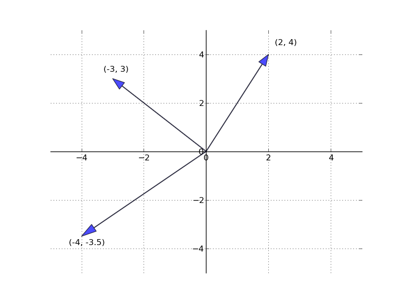
The set of all \(n\)-vectors is denoted \(\mathbb{R}^n\). For example, \(\mathbb{R}^2\) is the plane, and a vector in \(\mathbb{R}^2\) is just a point on that plane.

Vectors in the plane

2.2 Vectors in Julia

Julia is built with vectors and matrices as fundamental building blocks, making it a natural language for linear algebra. We begin by loading the LinearAlgebra standard library, which provides many of the functions we will use:

using LinearAlgebra

A simple vector can be created with square brackets:

x = [1., 2.]

2-element Vector{Float64}:
 1.0
 2.0

Julia provides several convenience functions for constructing common vectors:

x = zeros(3)           # A vector in R^3 filled with zeros
println("x = $x")
y = ones(4)            # A vector in R^4 filled with ones
println("y = $y")
z = collect(LinRange(0, 1, 6))  # 6 evenly spaced values between 0 and 1
println("z = $z")

x = [0.0, 0.0, 0.0]
y = [1.0, 1.0, 1.0, 1.0]
z = [0.0, 0.2, 0.4, 0.6, 0.8, 1.0]

The zeros and ones functions are especially common in numerical work. You will often initialize a vector of zeros and then fill in computed values, or use a vector of ones to construct a design matrix for regression (as we will see later in these notes).

2.2.1 Editing Vectors

Once a vector is created, you can edit individual elements using square-bracket indexing:

x[1] = 1
x

3-element Vector{Float64}:
 1.0
 0.0
 0.0

You can also access multiple elements at once using slice notation:

println(x[2:3])

[0.0, 0.0]

2.2.2 Assigning to Slices

When assigning values to a slice of a vector, you must use .= (the “dot-equals” operator) rather than plain =. The dot tells Julia to perform the assignment element-wise:

x[2:3] = 3, 4  # This produces an error

ArgumentError: indexed assignment with a single value to possibly many locations is not supported; perhaps use broadcasting `.=` instead?
Stacktrace:
 [1] setindex_shape_check(::Tuple{Int64, Int64}, ::Int64)
   @ Base ./indices.jl:276
 [2] _unsafe_setindex!(::IndexLinear, A::Vector{Float64}, x::Tuple{Int64, Int64}, I::UnitRange{Int64})
   @ Base ./multidimensional.jl:1017
 [3] _setindex!
   @ ./multidimensional.jl:1008 [inlined]
 [4] setindex!(A::Vector{Float64}, v::Tuple{Int64, Int64}, I::UnitRange{Int64})
   @ Base ./abstractarray.jl:1443
 [5] top-level scope
   @ ~/University of Oregon Dropbox/David Evans/University of Oregon/Courses/Spring 2026/EC 410/Lectures and Website/Julia/Linear Algebra/Linear Algebra Notes.qmd:116

x[2:3] .= 3, 4  # This works: assigns element-wise
x

3-element Vector{Float64}:
 1.0
 3.0
 4.0

This is our first encounter with Julia’s dot syntax for element-wise operations, which we will see much more of below.

2.3 Vector Operations

2.3.1 Addition

When we add two vectors, we add them element by element:

\[ x + y = \left[ \begin{array}{c} x_1 \\ x_2 \\ \vdots \\ x_n \end{array} \right] + \left[ \begin{array}{c} y_1 \\ y_2 \\ \vdots \\ y_n \end{array} \right] := \left[ \begin{array}{c} x_1 + y_1 \\ x_2 + y_2 \\ \vdots \\ x_n + y_n \end{array} \right] \]

Both vectors must have the same length for addition to be defined.

x = ones(3)
y = [2, 4, 6]
x + y

3-element Vector{Float64}:
 3.0
 5.0
 7.0

2.3.2 Scalar Multiplication

Scalar multiplication takes a scalar (a single number) \(\gamma\) and a vector \(x\), and multiplies every element by \(\gamma\):

\[ \gamma x := \left[ \begin{array}{c} \gamma x_1 \\ \gamma x_2 \\ \vdots \\ \gamma x_n \end{array} \right] \]

4*x

3-element Vector{Float64}:
 4.0
 4.0
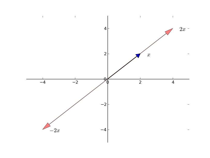
 4.0

Geometrically, scalar multiplication stretches or shrinks a vector (and flips its direction if \(\gamma < 0\)). Together with addition, these two operations define the structure of a vector space.

Vector addition and scalar multiplication

2.3.3 Element-wise Multiplication

In addition to scalar multiplication, we can multiply two vectors element by element using the .* operator:

println(x, y)
xy = x .* y

[1.0, 1.0, 1.0][2, 4, 6]

3-element Vector{Float64}:
 2.0
 4.0
 6.0

TipThe Dot Operator

In Julia, prefixing any operator with . applies it element-wise. This works with any function or operator: .+, .-, .*, ./, .^, and even f.(x) for any function f. This is called broadcasting and is a useful feature for numerical computing.

2.3.4 Inner Products and Norms

The inner product (or dot product) of two vectors \(x, y \in \mathbb{R}^n\) is defined as:

\[ x' y := \sum_{i=1}^n x_i y_i \]

The inner product measures how “aligned” two vectors are. Two vectors are orthogonal (perpendicular) if their inner product is zero.

The norm of a vector \(x\) represents its “length” or magnitude:

\[ \| x \| := \sqrt{x' x} := \left( \sum_{i=1}^n x_i^2 \right)^{1/2} \]

This is the Euclidean distance from the origin to the point \(x\). Norms are important in optimization and statistics—for example, least-squares regression works by minimizing the norm of a residual vector.

# Two ways to compute the inner product
println(sum(x .* y))   # Manual: element-wise multiply, then sum
println(dot(x, y))     # Built-in function from LinearAlgebra

12.0
12.0

# Two ways to compute the norm
println(sqrt(dot(x, x)))   # Manual: sqrt of inner product with itself
println(norm(x))            # Built-in function

1.7320508075688772
1.7320508075688772

# An example of orthogonal vectors
z = [-1., 2., -1]
println(dot(x, z))    # Zero: x and z are orthogonal

0.0

3 Spanning and Linear Independence

3.1 Linear Combinations and Span

Given a set of vectors \(A = \{a_1, \ldots, a_k\} \subset \mathbb{R}^n\), a natural question is: what new vectors can we create by combining these using addition and scalar multiplication? A vector \(y \in \mathbb{R}^n\) is a linear combination of \(A\) if there exist scalars \(\beta_1, \ldots, \beta_k\) such that:

\[ y = \beta_1 a_1 + \beta_2 a_2 + \ldots + \beta_k a_k \]

The set of all vectors that can be expressed as linear combinations of \(A\) is called the span of \(A\).

Linear combinations of two vectors span a plane

The concept of span tells us what part of \(\mathbb{R}^n\) is “reachable” from a given set of vectors.

3.1.1 Examples

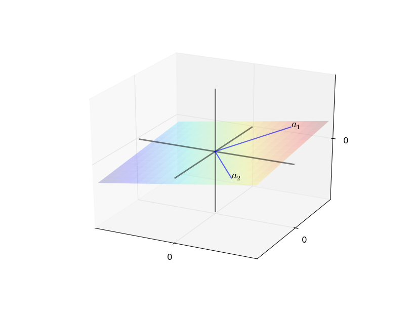
If \(A\) contains only a single vector \(a_1 \in \mathbb{R}^n\), then its span is the line through \(a_1\) and the origin—all scalar multiples \(\beta a_1\).

A more important example is the canonical basis for \(\mathbb{R}^n\). These are the \(n\) vectors:

\[ e_1 = \left[\begin{matrix}1\\0\\\vdots\\0\end{matrix}\right],\quad e_2 = \left[\begin{matrix}0\\1\\\vdots\\0\end{matrix}\right],\quad\ldots,\quad e_n = \left[\begin{matrix}0\\0\\\vdots\\1\end{matrix}\right] \]

The span of \(\{e_1, e_2, \ldots, e_n\}\) is all of \(\mathbb{R}^n\), because for any vector \(x \in \mathbb{R}^n\) we can write:

\[ x = x_1 e_1 + x_2 e_2 + \ldots + x_n e_n \]

That is, any vector is a linear combination of the canonical basis vectors, with the components of \(x\) serving as the coefficients.

3.1.2 A Counterexample

Not every collection of \(n\) vectors spans \(\mathbb{R}^n\). Consider \(A_0 = \{e_1, e_2, e_1 + e_2\} \subset \mathbb{R}^3\). If \(y = (y_1, y_2, y_3)\) is a linear combination of these vectors, then the third component must satisfy \(y_3 = 0\). So \(A_0\) fails to span all of \(\mathbb{R}^3\)—it only reaches the plane where the third coordinate is zero.

ImportantKey Insight

Adding more vectors to a set does not always increase the span. The new vector must point in a “genuinely new direction”—one that is not already reachable as a linear combination of the existing vectors.

3.2 Linear Independence

The counterexample above motivates the concept of linear independence. A set of vectors \(A = \{a_1, \ldots, a_k\} \subset \mathbb{R}^n\) is linearly dependent if some strict subset of \(A\) has the same span as \(A\) itself. Equivalently, at least one vector in the set can be written as a linear combination of the others—it is “redundant.” The set \(A\) is linearly independent if no such redundancy exists.

There are several equivalent ways to define linear independence:

1. No vector in \(A\) can be formed as a linear combination of the others.
2. The only solution to \(\beta_1 a_1 + \ldots + \beta_k a_k = 0\) is \(\beta_1 = \cdots = \beta_k = 0\).

An important consequence: since \(\mathbb{R}^n\) can be spanned by \(n\) vectors (the canonical basis), any set of more than \(n\) vectors in \(\mathbb{R}^n\) must be linearly dependent. There simply is not “room” for more than \(n\) independent directions.

3.2.1 Unique Representations

A key property of linearly independent vectors is that they provide unique representations of every vector in their span. Suppose \(A = \{a_1, \ldots, a_k\}\) is linearly independent and some vector \(y\) can be written as:

\[ y = \beta_1 a_1 + \ldots + \beta_k a_k = \gamma_1 a_1 + \ldots + \gamma_k a_k \]

Subtracting one expression from the other gives:

\[ (\beta_1 - \gamma_1) a_1 + \cdots + (\beta_k - \gamma_k) a_k = 0 \]

By linear independence, the only way this sum can equal zero is if every coefficient is zero, which means \(\gamma_i = \beta_i\) for all \(i\). In other words, the representation is unique.

This property is essential in regression analysis: when we write \(y = X\beta + \varepsilon\) and the columns of \(X\) are linearly independent, there is a unique coefficient vector \(\beta\) that provides the best linear fit.

4 Matrices

4.1 Definition and Basic Properties

An \(n \times k\) matrix is a rectangular array of numbers with \(n\) rows and \(k\) columns:

\[ A = \left[ \begin{array}{cccc} a_{11} & a_{12} & \cdots & a_{1k} \\ a_{21} & a_{22} & \cdots & a_{2k} \\ \vdots & \vdots & & \vdots \\ a_{n1} & a_{n2} & \cdots & a_{nk} \end{array} \right] \]

We can also view \(A\) as a collection of \(k\) column vectors in \(\mathbb{R}^n\):

\[ A = \left[\begin{matrix}a_1 & a_2 & \cdots & a_k\end{matrix}\right] \quad\text{where}\quad a_i = \left[\begin{matrix} a_{1i}\\ a_{2i} \\\vdots \\ a_{ni}\end{matrix}\right] \]

This “columns as vectors” perspective turns out to be extremely useful. It connects matrices to the concepts of span and linear independence we just discussed: the column space of \(A\) is exactly the span of its column vectors.

Some terminology:

• A matrix with \(n = 1\) is a row vector; a matrix with \(k = 1\) is a column vector.
• A matrix with \(n = k\) is square.
• The transpose \(A'\) (also written \(A^T\)) is formed by swapping rows and columns: the element at position \((i,j)\) in \(A\) moves to position \((j,i)\) in \(A'\).

\[ A = \left[ \begin{array}{cccc} a_{11} & a_{12} & \cdots & a_{1k} \\ \vdots & \vdots & & \vdots \\ a_{n1} & a_{n2} & \cdots & a_{nk} \end{array} \right] \quad A' = \left[ \begin{array}{cccc} a_{11} & a_{21} & \cdots & a_{n1} \\ \vdots & \vdots & & \vdots \\ a_{1k} & a_{2k} & \cdots & a_{nk} \end{array} \right] \]

If \(A\) is \(n \times k\), then \(A'\) is \(k \times n\).

4.1.1 Matrices and Transpose in Julia

In Julia, matrices are created by separating elements with spaces (within a row) and semicolons (between rows):

A = [1 2 3;
     4 5 6]

2×3 Matrix{Int64}:
 1  2  3
 4  5  6

The transpose is written naturally with an apostrophe:

A'

3×2 adjoint(::Matrix{Int64}) with eltype Int64:
 1  4
 2  5
 3  6

4.2 Special Matrices

Several kinds of matrices come up so often that they have special names.

4.2.1 Symmetric Matrices

A square matrix is symmetric if \(A = A'\)—that is, \(a_{ij} = a_{ji}\) for all \(i\) and \(j\). Symmetric matrices arise naturally in economics: variance-covariance matrices, Hessian matrices of utility functions, and input-output matrices are all symmetric (or can be made so).

A = [1 2; 2 1]

2×2 Matrix{Int64}:
 1  2
 2  1

A'    # Same as A

2×2 adjoint(::Matrix{Int64}) with eltype Int64:
 1  2
 2  1

4.2.2 Diagonal Matrices

A matrix is diagonal if the only nonzero entries lie on the principal diagonal (positions where the row index equals the column index: \(a_{11}, a_{22}, \ldots\)). The diag function extracts the diagonal of a matrix, and diagm constructs a diagonal matrix:

A = [1 2;
     3 4]

2×2 Matrix{Int64}:
 1  2
 3  4

diag(A)    # Extract the diagonal elements

2-element Vector{Int64}:
 1
 4

diagm(0 => [1, 2, 3])    # Create a 3×3 diagonal matrix

3×3 Matrix{Int64}:
 1  0  0
 0  2  0
 0  0  3

The 0 => syntax specifies which diagonal to place the values on. The main diagonal is 0; 1 is one above, -1 is one below:

diagm(1 => [1, 2, 3])    # Values on the first super-diagonal

4×4 Matrix{Int64}:
 0  1  0  0
 0  0  2  0
 0  0  0  3
 0  0  0  0

4.2.3 The Identity Matrix

The most important diagonal matrix is the identity matrix \(I\), which has ones on the diagonal and zeros everywhere else:

diagm(0 => ones(3))

3×3 Matrix{Float64}:
 1.0  0.0  0.0
 0.0  1.0  0.0
 0.0  0.0  1.0

The identity matrix can also be written in terms of the canonical basis vectors:

\[ I = \left[\begin{matrix}e_1 & e_2 & \cdots & e_n\end{matrix}\right] \]

Its key property—that it acts as the “multiplicative identity” for matrices, i.e. 1 for matrices—will become clear once we define matrix multiplication below.

4.3 Matrix Operations

4.3.1 Addition and Scalar Multiplication

Matrix addition and scalar multiplication work exactly as you would expect from vectors—element by element. For addition, both matrices must have the same dimensions (\(n \times k\)). For scalar multiplication, every element is multiplied by the scalar \(\gamma\):

\[ \gamma A := \left[ \begin{array}{ccc} \gamma a_{11} & \cdots & \gamma a_{1k} \\ \vdots & & \vdots \\ \gamma a_{n1} & \cdots & \gamma a_{nk} \end{array} \right] \]

A = [1 2; 3 4]
B = diagm(0 => ones(2))
2*A

2×2 Matrix{Int64}:
 2  4
 6  8

A + B

2×2 Matrix{Float64}:
 2.0  2.0
 3.0  5.0

4.3.2 Matrix Multiplication

Matrix multiplication is the central operation of linear algebra, and it is not element-wise. The \((i, j)\)-th element of the product \(AB\) is the inner product of row \(i\) of \(A\) with column \(j\) of \(B\):

How matrix multiplication works: row \(i\) of \(A\) dotted with column \(j\) of \(B\)

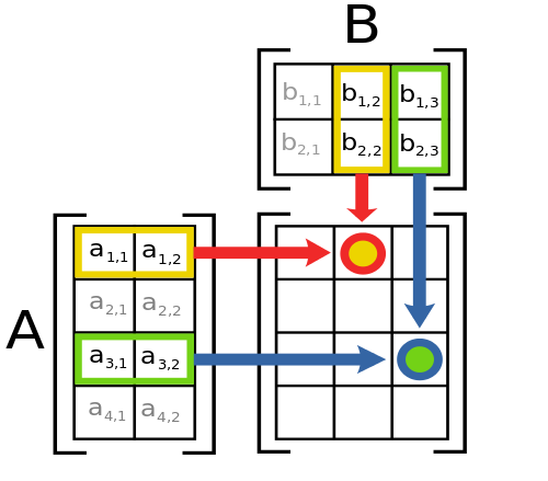
For the product \(AB\) to be defined, \(A\) must be \(n \times k\) and \(B\) must be \(k \times m\) (the “inner dimensions” must match). The result is an \(n \times m\) matrix.

An important fact: in general, \(AB \neq BA\). Matrix multiplication is not commutative. (This is analogous to why Julia uses * for string concatenation—both are non-commutative operations.)

4.3.3 Matrix-Vector Multiplication

A special case of matrix multiplication arises when we multiply an \(n \times k\) matrix \(A\) by a \(k \times 1\) vector \(x\), producing an \(n \times 1\) vector:

\[ Ax = \left[ \begin{array}{c} a_{11} x_1 + \cdots + a_{1k} x_k \\ \vdots \\ a_{n1} x_1 + \cdots + a_{nk} x_k \end{array} \right] \]

There is a beautiful alternative way to read this. If \(a_1, \ldots, a_k\) are the columns of \(A\), then:

\[ Ax = x_1 a_1 + x_2 a_2 + \ldots + x_k a_k \]

In other words, \(Ax\) is a linear combination of the columns of \(A\), with the entries of \(x\) as weights. This means \(Ax\) always lies in the span (or column space) of \(A\). This perspective is the key to understanding when systems of equations have solutions.

We can now state the defining property of the identity matrix: \(IA = A = AI\) for any conformable matrix \(A\). The identity matrix is the matrix equivalent of multiplying by 1.

4.3.4 Matrix Multiplication in Julia

In Julia, matrix multiplication uses the * operator:

A = [1 2; 3 4]

2×2 Matrix{Int64}:
 1  2
 3  4

I2 = diagm(0 => ones(2))

2×2 Matrix{Float64}:
 1.0  0.0
 0.0  1.0

A * I2    # Multiplying by the identity returns A

2×2 Matrix{Float64}:
 1.0  2.0
 3.0  4.0

4.3.5 Element-wise vs. Matrix Multiplication

It is crucial to distinguish between matrix multiplication (*) and element-wise multiplication (.*):

A .* I2    # Element-wise: very different from A * I2

2×2 Matrix{Float64}:
 1.0  0.0
 0.0  4.0

Julia also provides a built-in identity matrix object I that automatically conforms to the correct size:

A * I    # No need to construct an explicit identity matrix

2×2 Matrix{Int64}:
 1  2
 3  4

4.4 Broadcasting

Broadcasting is Julia’s mechanism for applying operations across arrays of different shapes. It replicates smaller arrays to match the dimensions of larger ones, all without actually creating copies in memory. The syntax uses the dot prefix (.).

A = diagm(0 => ones(2))

2×2 Matrix{Float64}:
 1.0  0.0
 0.0  1.0

b = [1, 2]

2-element Vector{Int64}:
 1
 2

A .+ b    # Adds b to each column of A

2×2 Matrix{Float64}:
 2.0  1.0
 2.0  3.0

Broadcasting follows a simple set of rules. Julia compares array shapes element-wise, starting from the trailing (rightmost) dimensions. Two dimensions are compatible when:

1. They are equal, or
2. One of them has length 1.

For example, consider arrays with the following shapes:

A      (4d array):  8 × 1 × 6 × 1
B      (3d array):      7 × 1 × 5
Result (4d array):  8 × 7 × 6 × 5

These are compatible because each pair of dimensions either matches or one is 1. But the following pair is not compatible:

A      (2d array):      2 × 1
B      (3d array):  8 × 4 × 3

The second dimensions (2 and 4) are neither equal nor 1, so broadcasting fails. Understanding these rules will save you from cryptic dimension-mismatch errors.

5 Solving Systems of Equations

5.1 Matrix Formulation

With vectors and matrices in hand, we can now express our original system of equations compactly. The system:

\[ \begin{array}{c} y_1 = a_{11} x_1 + a_{12} x_2 + \cdots + a_{1k} x_k \\ \vdots \\ y_n = a_{n1} x_1 + a_{n2} x_2 + \cdots + a_{nk} x_k \end{array} \]

can be written as a single matrix equation: \(y = Ax\).

Since \(Ax = x_1 a_1 + \ldots + x_k a_k\) is a linear combination of the columns of \(A\), the equation \(y = Ax\) has a solution only if \(y\) lies in the span (column space) of \(A\). If the columns of \(A\) are linearly independent and span all of \(\mathbb{R}^n\), then a unique solution exists for every \(y\). In this case we say \(A\) has full column rank.

The nature of the solution depends on the shape of \(A\):

• Square case (\(n = k\), full rank): exactly one solution.
• Over-determined (\(n > k\)): more equations than unknowns; typically no exact solution, but a best approximation exists.
• Under-determined (\(n < k\)): fewer equations than unknowns; infinitely many solutions.

Let us examine each case.

5.2 The Regular (Square) Case

When \(A\) is \(n \times n\) with linearly independent columns, the equation \(y = Ax\) has a solution for every \(y \in \mathbb{R}^n\), and this solution is unique. Define \(g(y)\) as the function that maps each \(y\) to its solution: \(y = Ag(y)\).

This function \(g\) turns out to be linear:

\[ g(\alpha w + \beta z) = \alpha g(w) + \beta g(z) \]

Since any linear function from \(\mathbb{R}^n\) to \(\mathbb{R}^n\) can be represented by a matrix, there exists a matrix \(A^{-1}\) such that \(g(y) = A^{-1} y\). This matrix is called the inverse of \(A\), and it satisfies:

\[ I = A^{-1}A = A A^{-1} \]

To solve \(y = Ax\), we simply pre-multiply both sides by \(A^{-1}\):

\[ A^{-1} y = A^{-1} A x = Ix = x \]

ImportantKey Result

When \(A\) is square and invertible, the solution to \(y = Ax\) is \(x = A^{-1}y\).

Not every square matrix has an inverse. The determinant provides a test: if \(\det(A) \neq 0\), then \(A\) is invertible (its columns are linearly independent). If \(\det(A) = 0\), the columns are linearly dependent, and no inverse exists.

5.2.1 Solving in Julia: The Inverse

A = [1 2; 3 4]
y = ones(2)
det(A)    # Check that det(A) ≠ 0

-2.0

A_inv = inv(A)

2×2 Matrix{Float64}:
 -2.0   1.0
  1.5  -0.5

x = A_inv * y

2-element Vector{Float64}:
 -0.9999999999999998
  0.9999999999999999

A * x    # Verify: should return y

2-element Vector{Float64}:
 1.0
 1.0000000000000004

5.2.2 Solving in Julia: The Backslash Operator

Julia provides the backslash operator \ as a more efficient and numerically stable way to solve \(Ax = y\):

x = A \ y

2-element Vector{Float64}:
 -1.0
  1.0

TipBest Practice

Prefer A \ y over inv(A) * y for solving systems. The backslash operator is more numerically stable (less sensitive to rounding errors) and more efficient (it avoids explicitly computing the inverse, which is an expensive operation). Computing the full inverse and then multiplying is rarely necessary in practice.

5.3 Over-determined Systems

When \(A\) is \(n \times k\) with \(n > k\)—more equations than unknowns—the system is over-determined. This is the case that arises in least-squares regression: we have more data points than parameters, and we want to find the parameter vector that provides the best fit.

In general, an arbitrary \(y \in \mathbb{R}^n\) will not lie in the span of \(A\) (which is at most \(k\)-dimensional in an \(n\)-dimensional space), so no exact solution exists. Instead, we look for the \(x\) that minimizes the distance between \(y\) and \(Ax\):

\[ \hat{x} = \arg\min_x \| y - Ax \| \]

When \(A\) has full column rank, the solution is given by the normal equations:

\[ \hat{x} = (A'A)^{-1}A'y \]

This is precisely the OLS (Ordinary Least Squares) estimator from econometrics. The matrix \((A'A)^{-1}A'\) is called the pseudo-inverse of \(A\), and Julia provides it via the pinv function.

5.3.1 Example: Fitting a Line

Suppose we want to fit a line \(y = mx + c\) through some noisy data:

x = [0, 1, 2, 3]
y = [-1, 0.2, 0.9, 2.1]

4-element Vector{Float64}:
 -1.0
  0.2
  0.9
  2.1

We rewrite this as a matrix equation \(y = Ap\) where \(A = [x \;\; \mathbf{1}]\) is the design matrix and \(p = [m \;\; c]'\) is the parameter vector:

A = [x ones(length(x))]

4×2 Matrix{Float64}:
 0.0  1.0
 1.0  1.0
 2.0  1.0
 3.0  1.0

The least-squares solution is:

m, c = pinv(A) * y
print(m, c)

1.0000000000000002-0.9499999999999998

We can verify this matches the normal equations formula \((A'A)^{-1}A'y\):

(A' * A) \ A' * y

2-element Vector{Float64}:
  0.9999999999999998
 -0.9499999999999996

5.3.2 Plotting the Fit

using Plots

scatter(x, y, label="Original data", markersize=10)
plot!(x, m*x .+ c, color=:red, label="Fitted line")

This is the essence of linear regression: find the line (or hyperplane) that minimizes the sum of squared residuals. The tools we have built up—vectors, matrices, inner products, norms, and the pseudo-inverse—provide both the mathematical foundation and the computational machinery.

5.4 Under-determined Systems

When \(A\) is \(n \times k\) with \(n < k\)—fewer equations than unknowns—the system is under-determined. In this case, we expect either no solutions (if \(y\) is not in the column space of \(A\)) or infinitely many solutions.

To understand why there are infinitely many solutions, consider the kernel (or null space) of \(A\): the set of all vectors \(\hat{x}\) such that \(A\hat{x} = 0\). If \(x\) is any solution to \(y = Ax\) and \(\hat{x}\) is in the kernel, then \(x + \hat{x}\) is also a solution:

\[ A(x + \hat{x}) = Ax + A\hat{x} = y + 0 = y \]

So we can add any kernel element to a known solution and get another valid solution. When the system is under-determined, the kernel is nontrivial (it contains nonzero vectors), giving us infinitely many solutions.

WarningCaution

Under-determined systems have infinitely many solutions. Methods like pinv return the minimum-norm solution—the solution with the smallest \(\|x\|\). Depending on the problem, this may or may not be the most economically meaningful solution. In structural estimation, additional restrictions (theory, moment conditions, etc.) are typically imposed to pin down a unique solution.

6 Eigenvalues and Eigenvectors

6.1 Definition

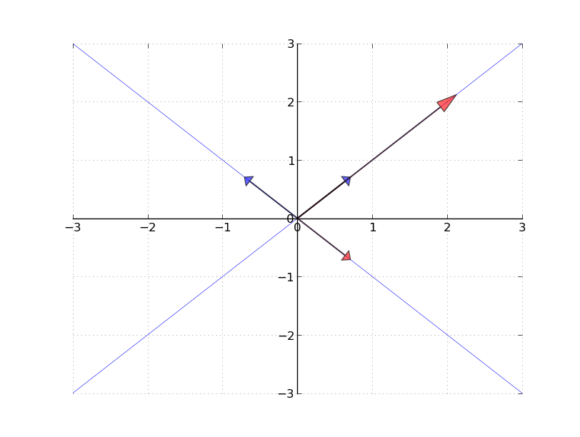
For a square \(n \times n\) matrix \(A\), we are interested in finding scalar \(\lambda\) and nonzero vector \(v \in \mathbb{R}^n\) such that:

\[ Av = \lambda v \]

When this equation holds, \(v\) is called an eigenvector of \(A\) and \(\lambda\) is the corresponding eigenvalue. The operation \(Av\) simply scales \(v\) by \(\lambda\)—the matrix acts like scalar multiplication along the direction of \(v\).

An eigenvector \(v\) is only scaled (not rotated) when multiplied by \(A\)

Eigenvalues and eigenvectors are fundamental in economics. They determine the stability of dynamic systems (e.g., whether a Solow model converges to its steady state), characterize principal components in data analysis, and play a central role in spectral methods for solving dynamic programming problems.

6.2 Finding Eigenvalues

To find eigenvalues, we rearrange \(Av = \lambda v\) as:

\[ 0 = Av - \lambda v = (A - \lambda I)v \]

For this equation to have a nonzero solution \(v\), the matrix \(A - \lambda I\) must have linearly dependent columns. This happens precisely when:

\[ \det(A - \lambda I) = 0 \]

The expression \(\det(A - \lambda I)\) is a polynomial of degree \(n\) in \(\lambda\), called the characteristic polynomial. Its roots are the eigenvalues.

6.3 Properties of Eigenvalues

Several useful facts connect eigenvalues to other matrix properties:

1. The determinant of \(A\) equals the product of its eigenvalues: \(\det(A) = \lambda_1 \cdot \lambda_2 \cdots \lambda_n\).
2. The trace of \(A\) (sum of diagonal elements) equals the sum of its eigenvalues: \(\text{tr}(A) = \lambda_1 + \lambda_2 + \cdots + \lambda_n\).
3. If \(A\) is symmetric, all eigenvalues are real (not complex).
4. If \(A\) is invertible with eigenvalues \(\lambda_1, \ldots, \lambda_n\), then \(A^{-1}\) has eigenvalues \(1/\lambda_1, \ldots, 1/\lambda_n\).

Property 1 gives us another way to check invertibility: \(A\) is invertible if and only if none of its eigenvalues are zero. Property 3 is especially useful because symmetric matrices arise so often in economics (variance-covariance matrices, Hessians of symmetric loss functions, etc.).

6.4 Eigenvalues in Julia

Julia makes eigenvalue computation straightforward with the eigen function:

A = [1 2; 2 1];
evals, evecs = eigen(A)

Eigen{Float64, Float64, Matrix{Float64}, Vector{Float64}}
values:
2-element Vector{Float64}:
 -1.0
  3.0
vectors:
2×2 Matrix{Float64}:
 -0.707107  0.707107
  0.707107  0.707107

evals    # The eigenvalues

2-element Vector{Float64}:
 -1.0
  3.0

evecs    # The eigenvectors (as columns)

2×2 Matrix{Float64}:
 -0.707107  0.707107
  0.707107  0.707107

TipReading the Output

The columns of evecs are the eigenvectors, and they correspond to the eigenvalues in evals in the same order. So the first column of evecs is the eigenvector for evals[1], and so on.

7 Economics Applications

The linear algebra tools we have developed—systems of equations, matrix inverses, eigenvalues, and decompositions—are not merely abstract mathematics. They are the computational backbone of much of applied economics. In this section, we work through two applications that illustrate how linear algebra appears in different branches of the field: input-output analysis (macroeconomics and trade) and OLS regression (econometrics)

7.1 Input-Output Model (Leontief)

7.1.1 Setup

In 1973, Wassily Leontief won the Nobel Prize in Economics for developing input-output analysis, a framework for studying the interdependencies between industries in an economy. The key idea is simple: to produce steel, you need coal and iron ore; to produce cars, you need steel, rubber, and glass; and the coal industry itself needs some steel (for mining equipment). Every industry is both a producer and a consumer of other industries’ output.

Consider an economy with \(n\) industries. Let \(a_{ij}\) denote the amount of good \(i\) required to produce one unit of good \(j\). These coefficients form the \(n \times n\) input-output matrix (or technology matrix) \(A\). Let \(x\) be the \(n \times 1\) vector of gross output (total production of each industry) and let \(d\) be the \(n \times 1\) vector of final demand (the output consumed by households, government, or exported—everything that is not used as an intermediate input).

The total output of each industry must satisfy two demands: intermediate demand from other industries (\(Ax\)) and final demand from consumers (\(d\)):

\[ x = Ax + d \]

Reading this equation column by column: the \(j\)-th column of \(Ax\) tells you how much of each good is needed as an input to produce \(x_j\) units of good \(j\). Summing across all industries and adding final demand gives the total demand for each good, which must equal total supply.

7.1.2 The Leontief Inverse

Rearranging the equation to solve for gross output:

\[ x - Ax = d \quad \Longrightarrow \quad (I - A)x = d \quad \Longrightarrow \quad x = (I - A)^{-1} d \]

The matrix \((I - A)^{-1}\) is called the Leontief inverse. It is one of the most important objects in input-output economics. The element in row \(i\), column \(j\) of \((I - A)^{-1}\) tells you the total amount of good \(i\) needed—both directly and indirectly through the entire supply chain—to deliver one additional unit of good \(j\) to final consumers.

Why “indirectly”? Suppose final demand for cars increases by one unit. The car industry needs more steel (a direct effect). But producing that extra steel requires more coal, and producing that extra coal requires more steel, and so on. The Leontief inverse captures this entire cascade of indirect effects, summing up the infinite chain of input requirements.

Mathematically, \((I - A)^{-1} = I + A + A^2 + A^3 + \cdots\) when the series converges. The term \(A^k\) captures the \(k\)-th round of indirect effects. The direct effect is \(I\) (one unit of the good itself), the first round of inputs is \(A\), the inputs needed to produce those inputs is \(A^2\), and so on.

ImportantWhen Does the Leontief Inverse Exist?

The system has a non-negative solution for any non-negative demand vector \(d\) if and only if \((I - A)\) is invertible and \((I - A)^{-1}\) has all non-negative entries. A sufficient condition is that the spectral radius of \(A\) (the largest absolute eigenvalue) is strictly less than 1. Economically, this means the economy is productive: each industry uses less than one unit of total inputs to produce one unit of output. If this condition fails, the economy cannot sustain itself: it consumes more than it produces.

7.1.3 A Three-Sector Example

Let us build a concrete example with three sectors: Agriculture (sector 1), Manufacturing (sector 2), and Services (sector 3).

# Input-output matrix: a_ij = amount of good i needed per unit of good j
# Columns: Agriculture, Manufacturing, Services
A_io = [0.10  0.20  0.05;    # Agriculture inputs
        0.15  0.10  0.10;    # Manufacturing inputs
        0.05  0.15  0.10]    # Services inputs

3×3 Matrix{Float64}:
 0.1   0.2   0.05
 0.15  0.1   0.1
 0.05  0.15  0.1

The first column tells us that producing one unit of agricultural output requires 0.10 units of agriculture itself (seeds, animal feed), 0.15 units of manufacturing (tractors, fertilizer), and 0.05 units of services (transportation, finance). The second column says that manufacturing requires 0.20 units of agriculture (cotton, food for workers), 0.10 of its own output, and 0.15 units of services. And so on.

First, let us verify that the economy is productive by checking the spectral radius:

evals_io = eigvals(A_io)
spectral_radius = maximum(abs.(evals_io))
println("Eigenvalues of A: $evals_io")
println("Spectral radius: $(round(spectral_radius, digits=4))")
println("Economy is productive: $(spectral_radius < 1)")

Eigenvalues of A: [-0.090670127121077, 0.05308993370463013, 0.337580193416447]
Spectral radius: 0.3376
Economy is productive: true

The spectral radius is less than 1, so the Leontief inverse exists and has non-negative entries. Now suppose final demand is \(d = (100, 200, 150)'\) (i.e. households want 100 units of agricultural goods, 200 units of manufactured goods, and 150 units of services). What gross output does each industry need to produce?

d = [100.0, 200.0, 150.0]    # Final demand

# Compute the Leontief inverse
leontief_inv = inv(I - A_io)
println("Leontief inverse:")
display(round.(leontief_inv, digits=4))

Leontief inverse:

3×3 Matrix{Float64}:
 1.1621  0.2741  0.095
 0.2046  1.1803  0.1425
 0.0987  0.2119  1.1401

# Gross output required
x = leontief_inv * d
println("\nFinal demand:  $d")
println("Gross output:  $(round.(x, digits=2))")
println("Intermediate:  $(round.(x .- d, digits=2))")

Final demand:  [100.0, 200.0, 150.0]
Gross output:  [185.27, 277.91, 223.28]
Intermediate:  [85.27, 77.91, 73.28]

Notice that gross output exceeds final demand for every sector. The difference \(x - d\) is the intermediate demand: the output that gets used up as inputs by other industries. Manufacturing, for example, must produce considerably more than the 200 units consumers want, because agriculture and services also need manufactured goods as inputs.

We can also ask: what happens if final demand for manufacturing increases by 50 units?

d_new = [100.0, 250.0, 150.0]    # Manufacturing demand up by 50
x_new = leontief_inv * d_new
println("Change in gross output: $(round.(x_new .- x, digits=2))")

Change in gross output: [13.7, 59.02, 10.6]

The change in gross output is exactly the second column of the Leontief inverse, scaled by 50. Every sector must increase production, not just manufacturing: this is the multiplier effect of input-output analysis.

7.2 OLS Regression

7.2.1 The Normal Equations

Ordinary Least Squares (OLS) is perhaps the most widely used statistical method in economics. We encountered the least-squares formula earlier when discussing over-determined systems. Here we develop the implementation more carefully, emphasizing the connection to the linear algebra tools we have built.

The regression model is \(y = X\beta + \varepsilon\), where \(y\) is an \(n \times 1\) vector of outcomes, \(X\) is an \(n \times k\) matrix of regressors (including a column of ones for the intercept), \(\beta\) is a \(k \times 1\) vector of coefficients, and \(\varepsilon\) is an \(n \times 1\) vector of errors. The OLS estimator minimizes the sum of squared residuals:

\[ \hat{\beta} = \arg\min_\beta \|y - X\beta\|^2 = (X'X)^{-1}X'y \]

7.2.2 Implementation

Let us generate simulated data with known true coefficients and verify that OLS recovers them:

using Random
Random.seed!(123) #This ensures the same random numbers are generated each time the code is run

n = 200          # Number of observations
β_true = [2.0, -1.5, 0.8]    # True coefficients: intercept, x₁, x₂
σ_ε = 1.0       # Standard deviation of errors

# Generate regressors
X_raw = randn(n, 2)                           # Two explanatory variables
X = hcat(ones(n), X_raw)                       # Add intercept column
ε = σ_ε * randn(n)                             # Error terms
y = X * β_true + ε                             # Observed outcomes

println("True β:      $β_true")

True β:      [2.0, -1.5, 0.8]

Now we estimate \(\hat{\beta}\) using both the explicit normal equations formula and the numerically superior backslash operator:

# Method 1: Normal equations (explicit formula)
β_hat_normal = inv(X' * X) * X' * y

# Method 2: Backslash operator (numerically stable)
β_hat_backslash = X \ y

println("β̂ (normal equations): $(round.(β_hat_normal, digits=4))")
println("β̂ (backslash):        $(round.(β_hat_backslash, digits=4))")
println("True β:               $β_true")

β̂ (normal equations): [2.065, -1.5256, 0.8382]
β̂ (backslash):        [2.065, -1.5256, 0.8382]
True β:               [2.0, -1.5, 0.8]

Both methods give the same answer (to many decimal places), but the backslash approach is preferred. To see why, consider what happens when the columns of \(X\) are nearly collinear. The matrix \(X'X\) becomes nearly singular, and inverting it amplifies rounding errors dramatically. The backslash operator uses a QR decomposition internally, which avoids forming \(X'X\) entirely and is therefore much more robust.

7.2.3 Standard Errors

To conduct inference, we need the standard errors of \(\hat{\beta}\). Under the classical assumptions (\(\varepsilon \sim N(0, \sigma_\varepsilon^2 I)\)), the variance-covariance matrix of \(\hat{\beta}\) is:

\[ \text{Var}(\hat{\beta}) = \hat{\sigma}^2 (X'X)^{-1} \]

where \(\hat{\sigma}^2 = \frac{1}{n - k} \|y - X\hat{\beta}\|^2\) is the estimated error variance (using the degrees-of-freedom correction \(n - k\)). The standard errors are the square roots of the diagonal elements.

k = size(X, 2)                           # Number of regressors
residuals = y - X * β_hat_backslash      # Residual vector
σ̂² = dot(residuals, residuals) / (n - k) # Estimated error variance
var_β = σ̂² * inv(X' * X)                 # Variance-covariance matrix
se_β = sqrt.(diag(var_β))                # Standard errors

println("Estimated coefficients and standard errors:")
for i in 1:k
    println("  β̂_$i = $(round(β_hat_backslash[i], digits=4)) ± $(round(se_β[i], digits=4))")
end
println("\nEstimated σ² = $(round(σ̂², digits=4))  (true σ² = $(σ_ε^2))")

Estimated coefficients and standard errors:
  β̂_1 = 2.065 ± 0.0698
  β̂_2 = -1.5256 ± 0.0716
  β̂_3 = 0.8382 ± 0.0671

Estimated σ² = 0.9675  (true σ² = 1.0)

Notice how the variance-covariance matrix \(\hat{\sigma}^2 (X'X)^{-1}\) combines two ideas from our linear algebra toolkit: the inverse of \(X'X\) (which captures how “spread out” the regressors are—more variation means more precise estimates) and the estimated noise level \(\hat{\sigma}^2\).

TipWhy Not Just Use a Package?

In practice, you would use a package like GLM.jl for regression analysis. The point of implementing OLS by hand is to see that the entire procedure—estimation, residuals, standard errors—is nothing but linear algebra: matrix multiplication, the inverse, and the dot product. Understanding the mechanics makes you a better consumer of regression output.

8 Summary

These notes covered the essential linear algebra concepts needed for computational economics:

Vectors are ordered sequences of numbers that live in \(\mathbb{R}^n\). We can add them, scale them, compute their inner products, and measure their lengths with norms.

Spanning and linear independence tell us about the structure of vector spaces. The span of a set of vectors is the set of all their linear combinations. Linearly independent vectors provide unique representations—a property essential for regression and identification.

Matrices generalize vectors to two dimensions. They represent linear transformations and systems of equations. Key operations include transpose, addition, scalar multiplication, and matrix multiplication (which is not element-wise and not commutative).

Solving systems depends on the shape of the matrix:

• Square, invertible (\(n = n\)): unique solution via \(x = A^{-1}y\) or A \ y.
• Over-determined (\(n > k\)): least-squares solution via \(\hat{x} = (A'A)^{-1}A'y\) or pinv(A) * y.
• Under-determined (\(n < k\)): infinitely many solutions; pinv returns the minimum-norm solution.

Eigenvalues and eigenvectors reveal the intrinsic structure of square matrices. They determine stability of dynamic systems and are connected to determinants and traces.

Economics applications tie these tools together. The Leontief input-output model uses matrix inversion to trace supply-chain interdependencies. OLS regression is a least-squares problem solved by the normal equations.

TipKey Julia Tools

Function	Purpose
dot(x, y)	Inner product
norm(x)	Vector norm
det(A)	Determinant
inv(A)	Matrix inverse
A \ y	Solve \(Ax = y\) (preferred)
pinv(A)	Pseudo-inverse (for least-squares)
eigen(A)	Eigenvalues and eigenvectors
isposdef(A)	Check positive definiteness
diag(A), diagm(...)	Extract/create diagonal matrices
.*, .+, etc.	Element-wise (broadcast) operations